pyplot01
pyplot01
pyplot 1
예제 6_1
test1 (자료 가져오기)
1
2
3
4
5
6
7
8
9
10
11
12
13
14
15
16
17
18
19
20
21
22
23
24
25
26
27
28
29
30
31
32
33
34
35
import numpy as np
import pandas as pd
from matplotlib import pyplot as plt

# 한글 폰트 사용을 위해서 세팅
from matplotlib import font_manager, rc
font_path = "NanumGothic.ttf"
font = font_manager.FontProperties(fname=font_path).get_name()
rc('font', family=font)
# import matplotlib as mpl
# mpl.matplotlib_fname()

def testplot1():
    ind_path = './indicators.csv'
    dt_ind = {
        'CountryName':np.unicode_,
        'CountryCode':np.unicode_,
        'IndicatorName':np.unicode_,
        'IndicatorCode':np.unicode_,
        'Year':np.int16,
        'Value':np.float64
    }
    df_ind = pd.read_csv(ind_path,dtype=dt_ind,sep=',')
    print(df_ind.head())
    print('========')

    uniq_countries = df_ind['CountryName'].unique()
    num_ctry = uniq_countries.shape[0]
    print('num of country :',num_ctry)
    print(len(uniq_countries))

    min_yr, max_yr = min(df_ind['Year']),max(df_ind['Year'])
    print('year',min_yr,'to',max_yr)

    return None
1
2
3
4
5
6
7
8
9
10
11
12
  CountryName CountryCode  ...  Year         Value
0  Arab World         ARB  ...  1960  1.335609e+02
1  Arab World         ARB  ...  1960  8.779760e+01
2  Arab World         ARB  ...  1960  6.634579e+00
3  Arab World         ARB  ...  1960  8.102333e+01
4  Arab World         ARB  ...  1960  3.000000e+06

[5 rows x 6 columns]
========
num of country : 247
247
year 1960 to 2015
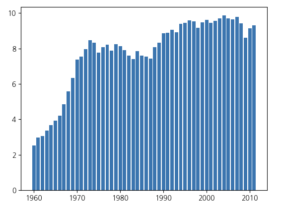
test2 (bar)
1
2
3
4
5
6
7
8
9
10
11
12
13
14
15
16
17
18
19
20
21
22
23
24
25
26
27
28
def testplot2():
    ind_path = './indicators.csv'
    dt_ind = {
        'CountryName':np.unicode_,
        'CountryCode':np.unicode_,
        'IndicatorName':np.unicode_,
        'IndicatorCode':np.unicode_,
        'Year':np.int16,
        'Value':np.float64
    }
    df_ind = pd.read_csv(ind_path,dtype=dt_ind,sep=',')

    # cond1 & cond2 ==> CO2 emission & korea
    ind_co2 = 'CO2 emissions \(metric'
    ctr_code = 'KOR'
    ctr_code2 = 'USA'
    ctr_code3 = 'JPN'
    cond1 = df_ind['IndicatorName'].str.contains(ind_co2)
    cond2 = df_ind['CountryCode'].str.contains(ctr_code3)
    res = df_ind[cond1 & cond2]
    #print(res.head())

    years = res['Year'].values
    co2 = res['Value'].values
    plt.bar(years,co2)
    plt.show()

    return None
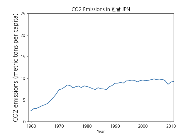
test3 (graph)
1
2
3
4
5
6
7
8
9
10
11
12
13
14
15
16
17
18
19
20
21
22
23
24
25
26
27
28
29
30
31
32
33
34
35
36
37
38
39
40
41
def testplot3():
    ind_path = './indicators.csv'
    dt_ind = {
        'CountryName':np.unicode_,
        'CountryCode':np.unicode_,
        'IndicatorName':np.unicode_,
        'IndicatorCode':np.unicode_,
        'Year':np.int16,
        'Value':np.float64
    }
    df_ind = pd.read_csv(ind_path,dtype=dt_ind,sep=',')

    # cond1 & cond2 ==> CO2 emission & korea
    ind_co2 = 'CO2 emissions \(metric'
    ctr_code = 'KOR'
    ctr_code2 = 'USA'
    ctr_code3 = 'JPN'
    code = ctr_code3
    cond1 = df_ind['IndicatorName'].str.contains(ind_co2)
    cond2 = df_ind['CountryCode'].str.contains(code)
    res = df_ind[cond1 & cond2]
    #print(res.head())

    years = res['Year'].values
    co2 = res['Value'].values

    # switch into a line chart
    plt.plot(years,co2)
    # coordination
    # xlabel, ylabel, title
    # label the axes
    plt.xlabel('Year')
    plt.ylabel(res['IndicatorName'].iloc[0],fontsize = 15)
    # label the graph
    plt.title('CO2 Emissions in 한글 ' + str(code))

    # 축 범위 설정
    plt.axis([1959,2011,0,25])
    plt.show()

    return None
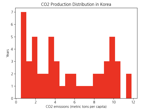
test4 (histogram)
1
2
3
4
5
6
7
8
9
10
11
12
13
14
15
16
17
18
19
20
21
22
23
24
25
26
27
28
29
30
31
32
33
34
35
36
37
38
39
40
41
def testplot4():
    ind_path = './indicators.csv'
    dt_ind = {
        'CountryName':np.unicode_,
        'CountryCode':np.unicode_,
        'IndicatorName':np.unicode_,
        'IndicatorCode':np.unicode_,
        'Year':np.int16,
        'Value':np.float64
    }
    df_ind = pd.read_csv(ind_path,dtype=dt_ind,sep=',')

    # cond1 & cond2 ==> CO2 emission & korea
    ind_co2 = 'CO2 emissions \(metric'
    ctr_code = 'KOR'
    ctr_code2 = 'USA'
    ctr_code3 = 'JPN'
    code = ctr_code
    cond1 = df_ind['IndicatorName'].str.contains(ind_co2)
    cond2 = df_ind['CountryCode'].str.contains(code)
    co2_res = df_ind[cond1 & cond2]
    #print(res.head())

    #years = res['Year'].values
    #co2 = res['Value'].values


    # 오차범위 내 값만 사용하기
    l_bnd = co2_res['Value'].mean() - co2_res['Value'].std()
    u_bnd = co2_res['Value'].mean() + co2_res['Value'].std()
    # extract values within error bnd
    #hgram_data = [x for x in co2_res[:10000]['Value'] if l_bnd <= x and x <= u_bnd]
    hgram_data = co2_res['Value'].values
    print(hgram_data)

    plt.hist(hgram_data,bins=20,density=False,histtype='bar',color='red')
    plt.xlabel(co2_res['IndicatorName'].iloc[0])
    plt.ylabel('Years')
    plt.title('CO2 Production Distribution in Korea')
    plt.show()
    return None
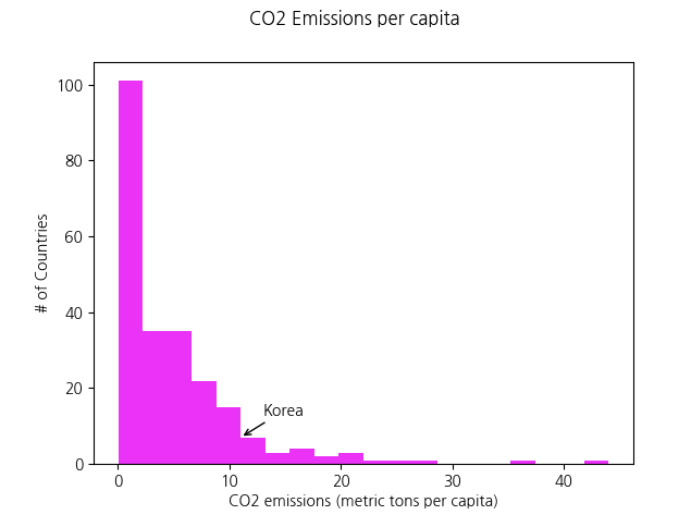
test5 (annotate)
1
2
3
4
5
6
7
8
9
10
11
12
13
14
15
16
17
18
19
20
21
22
23
24
25
26
27
28
29
30
31
32
33
34
35
36
37
38
39
def testplot5():
    ind_path = './indicators.csv'
    dt_ind = {
        'CountryName':np.unicode_,
        'CountryCode':np.unicode_,
        'IndicatorName':np.unicode_,
        'IndicatorCode':np.unicode_,
        'Year':np.int16,
        'Value':np.float64
    }
    df_ind = pd.read_csv(ind_path,dtype=dt_ind,sep=',')

    # cond1 & cond2 ==> CO2 emission & korea
    ind_co2 = 'CO2 emissions \(metric'
    years = [2011]

    cond1 = df_ind['IndicatorName'].str.contains(ind_co2)
    cond2 = df_ind['Year'].isin(years)
    CO2_2011_all = df_ind[cond1 & cond2]
    print(CO2_2011_all)

    fig, axis = plt.subplots() # 그래프를 여러개 넣을수 있음
    axis.set_xlabel(CO2_2011_all['IndicatorName'].iloc[0])
    axis.set_ylabel('# of Countries')
    #axis.set_title('CO2 Emissions per capita')
    axis.hist(CO2_2011_all['Value'],bins=20,density=False,color='magenta')
    fig.suptitle('CO2 Emissions per capita')

    # Annotating
    # ax.annotate(text,xy,xytext,xycoords,arrowprops)
    # text : the text of the annotation
    # xy: the point (x,y) to annotate
    # xytext : the point (x,y) of the text
    # xycoords : coordinate system
    # arrowprops : propertiex of arrow
    axis.annotate('Korea',(11,7),(13,13),xycoords='data',arrowprops=dict(arrowstyle = '->'))

    plt.show()
    return None
test6 (scatter & correlation)
1
2
3
4
5
6
7
8
9
10
11
12
13
14
15
16
17
18
19
20
21
22
23
24
25
26
27
28
29
30
31
32
33
34
35
36
37
38
39
40
41
42
43
def testplot6():
ind_path = './indicators.csv'
dt_ind = {
'CountryName':np.unicode_,
'CountryCode':np.unicode_,
'IndicatorName':np.unicode_,
'IndicatorCode':np.unicode_,
'Year':np.int16,
'Value':np.float64
}
df_ind = pd.read_csv(ind_path,dtype=dt_ind,sep=',')
# cond1 & cond2 ==> CO2 emission & korea
ind_co2 = 'CO2 emissions \(metric'
ctr_code = 'KOR'
ctr_code2 = 'USA'
input_ctr_code = ctr_code
cond1 = df_ind['IndicatorName'].str.contains(ind_co2)
cond2 = df_ind['CountryCode'].str.contains(input_ctr_code)
co2_res = df_ind[cond1 & cond2]
ind_gdp = 'GDP per capita \(constant 2005'
cond3 = df_ind['IndicatorName'].str.contains(ind_gdp)
cond2 = df_ind['CountryCode'].str.contains(input_ctr_code)
gdp_res = df_ind[cond3 & cond2]
gdp_res_to_2011 = gdp_res[gdp_res["Year"] < 2012]
#print(co2_res)
#print(gdp_res_to_2011)
fig, axis = plt.subplots() # 그래프를 여러개 넣을수 있음
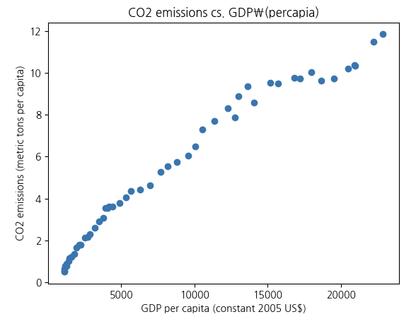
axis.set_title('CO2 emissions cs. GDP\(percapia)')
axis.set_xlabel(gdp_res_to_2011['IndicatorName'].iloc[0])
axis.set_ylabel(co2_res['IndicatorName'].iloc[0])
x_data = gdp_res_to_2011['Value'].values
y_data = co2_res['Value'].values
axis.scatter(x_data,y_data)
plt.show()
# correlation
R = np.corrcoef(x_data,y_data)
print(R)
return None
1
2
[[1.         0.98102799]
 [0.98102799 1.        ]]
test7 (boxplot)
1
2
3
4
5
6
7
8
9
10
11
12
13
14
15
16
17
18
19
20
21
22
23
24
25
26
27
28
29
30
31
32
33
34
35
36
37
38
39
40
41
42
43
44
45
46
def testplot7():
ind_path = './indicators.csv'
dt_ind = {
'CountryName':np.unicode_,
'CountryCode':np.unicode_,
'IndicatorName':np.unicode_,
'IndicatorCode':np.unicode_,
'Year':np.int16,
'Value':np.float64
}
df_ind = pd.read_csv(ind_path,dtype=dt_ind,sep=',')
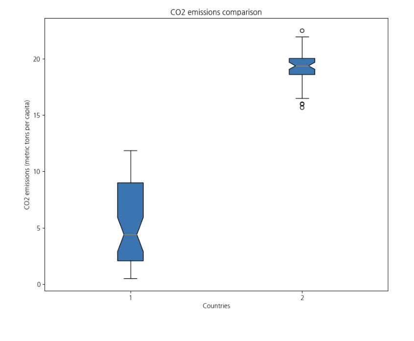
countries = ['KOR','USA']
ind_co2 = 'CO2 emissions \(metric'
cond_co2 = df_ind['IndicatorName'].str.contains(ind_co2)
df_co2 = df_ind[cond_co2]
cond_ctr = df_co2['CountryCode'].str.contains(countries[0])
co2_kor = df_co2[cond_ctr]['Value'].values
cond_ctr = df_co2['CountryCode'].str.contains(countries[1])
co2_usa = df_co2[cond_ctr]['Value'].values
co2_emissions = pd.DataFrame({'KOR':co2_kor,'USA':co2_usa})
fig, axis = plt.subplots(figsize = (10,8))
plt.boxplot(co2_emissions,notch=True,patch_artist=True)
plt.xlabel('Countries')
plt.ylabel(df_co2['IndicatorName'].iloc[0])
plt.title('CO2 emissions comparison')
plt.show()
return None
def main():
testplot1()
#testplot2()
#testplot3()
#testplot4()
#testplot5()
#testplot6()
#testplot7()
return None
if __name__ =='__main__':
main()
This post is licensed under CC BY 4.0 by the author.